Week 1 Review L01 - L03
Chapter 1: Signals and Amplifiers
- [[#1.1 Signals and Sources]]
- [[#1.2 Frequency Spectrum of Signals]]
- [[#1.3 Analog and Digital Signals]]
- [[#1.4 Amplifiers]]
- [[#1.5 Circuit Models for Amplifiers]]
[[#Chapter 2 Operational Amplifiers]]
1.1 Signals and Sources
Alternating Current (AC) is a time varying, sinusoidal signal.
e.g. Microphone
Direct Current (DC) is a static or fixed signal.
e.g. Battery
e.g. square wave and how you can break it up with fourier series
because ECE231 moved from winter semester to fall semester
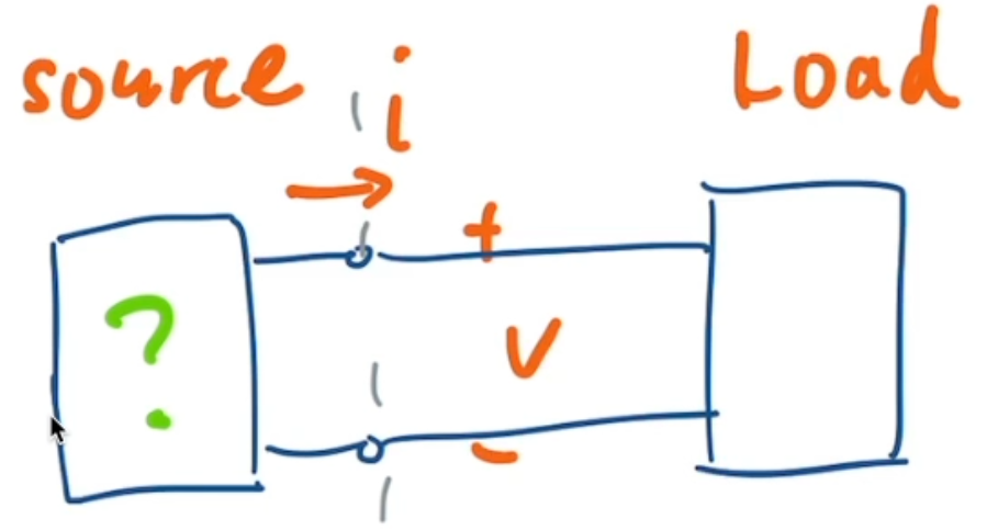
Recap: Relating Signals to Thevenin and Norton Equivalent Circuits
Let's think of a signal source as a "black box"
- It doesn't matter so much what is inside the box, but rather how it behaves outside the box.
- Has two terminals coming out of it, which shows us:
- Voltage
- Current coming in/out
- We connect this to a "load"
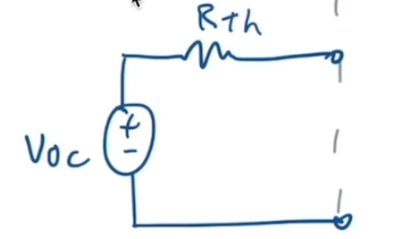
- Analogous to what you do with Thevenin/Norton; separating the "load" (usually a resistor) from the source (the Thevenin/Norton simplification).
Simplifying a circuit (or a portion of it) down to a voltage source in series with a resistor. We will use this the most in this course because most of the time we'll be dealing with voltages and voltage amplifiers.
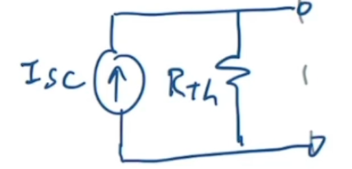
Simplifying a circuit (or a portion of it) down to a current source parallel to a resistor.
1.2 Frequency Spectrum of Signals
I don't think we're doing much of this at all in this course?
1.3 Analog and Digital Signals
"analog" like a physical voice, whereas "digital" is like the .mp4 file of a voice - stored as binary.
1.4 Amplifiers
Amplification is when a signal comes into a circuit and gets increased ("amplified"). Often we simplify this to a single triangle.
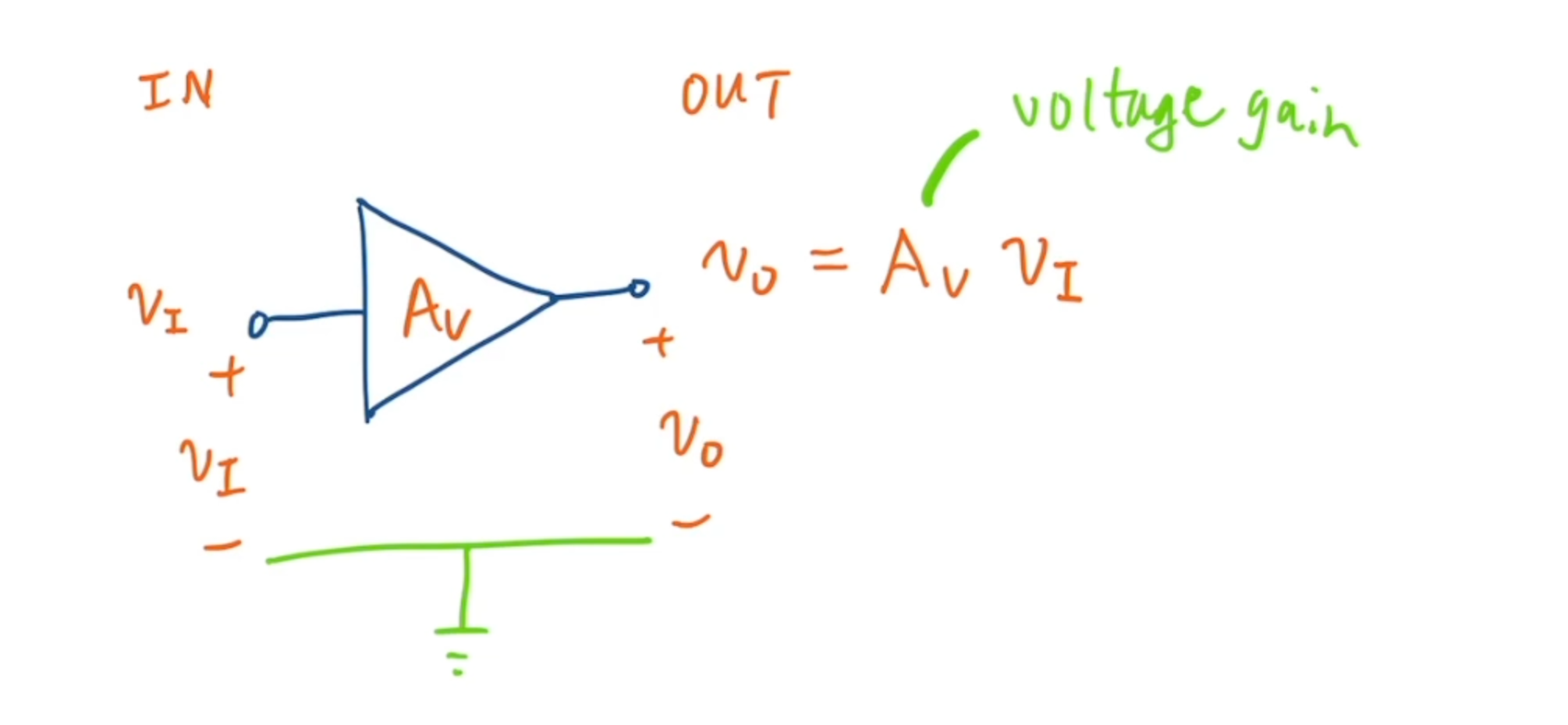
In the above image, the reference voltage is set to ground, i.e.,
Linear amplifier
A linear amplifier is an amplifier that amplifies linear, which is to say that the output voltage follows this equation:
1.5 Circuit Models for Amplifiers
"Direct extension of Thevenin's and Norton's" - Phang
Modelling a Linear Amplifier with Thevenin's Theorem
Given a "black box" circuit (i.e., one that has a source connected to a load), we can model it using Thevenin's Theorem, as long as it is linear. Thus, we can also model a linear amplifier using a Thevenin circuit.
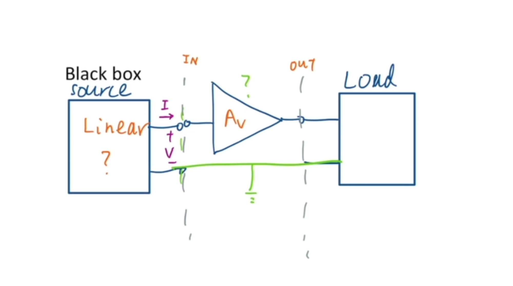
The input side of the amplifier can be modelled as a resistor (since it is a linear input), which comes from the linear source (left side of the above image). We can do this because it's a Thevenin simplification, i.e., simplified to a resistor and a voltage.
Then, since we know that
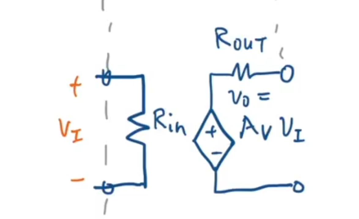
This then gets you three parameters:
: Input resistance (source, e.g. a battery) : output resistance (load, e.g. an LED) : voltage gain of the amplifier
Amplifier Types
- Voltage amplifier -> gain is
- Gain will be very large (
)
- Gain will be very large (
- Current amplifier -> gain is
- Power amplifier -> gain is
- Note that a power amplifier is mostly just current amplification usually.
Decibel (dB) Scale
Since the voltage gain in a voltage amplifier is so large, we, by convention, use dB to discuss voltage gain. So:
- Voltage gain in dB expressed as
- Current gain in dB expressed as
- Power gain in dB expressed as
- This is because:
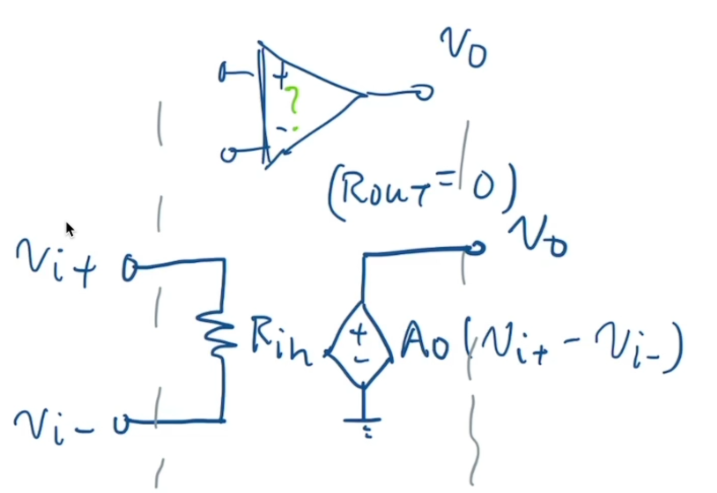
Chapter 2: Operational Amplifiers
2.1 The Ideal Op Amp
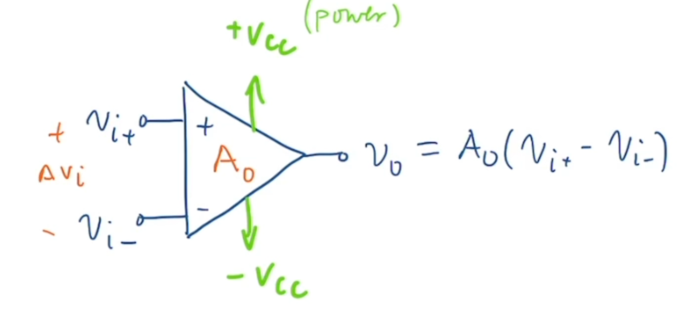
The Operational Amplifier:
- Takes in an inverting input voltage
, as well as a noninverting input voltage is called the noninverting input voltage because it has the same sign as the output, whereas has the opposite sign. - In the circuit model of an operational amplifier,
is distinguished by a sign in the triangle symbol, and is distinguished by a sign.
- Outputs an output voltage that follows this equation (i.e., it scales the difference between the input voltages linearly):
- Has two DC power terminals (
) added because it contains semiconductors - Output voltage cannot be scaled more than
.
- Output voltage cannot be scaled more than
- Rejects common signals
- e.g. if
, then ideally . - This is known as common-mode rejection
- e.g. if
e.g.
The output voltage
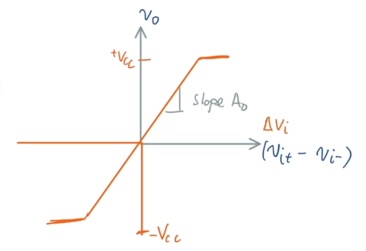
The ideal operational amplifier has:
- Zero input current, i.e. doesn't "bleed" any current to amplify voltage
- Zero output resistance, i.e. zero load voltage
- Infinite op-amp gain:
- This implies that your
slope will basically go straight up.
- This implies that your
Circuit Model of the Ideal Operational Amplifier
As with the linear amplifier from [[#1.5 Circuit Models for Amplifiers]], we can model the operational amplifier as a circuit - the main difference being that there are two input voltages modelled around the input resistor instead of one.